
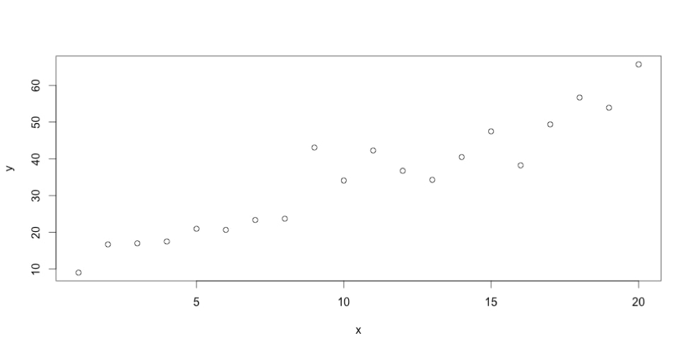
x<-seq(1,20,1)noise<-rnorm(20,0,5)y<-2.38*x+8.29 + noiseplot(x,y)Here's what the plot looks like:
 Now let’s see how to fit a line through these points with the Nelder-Mead optimization algorithm. Nelder-Mead works by drawing smaller and smaller areas with different values for the parameters, until they converge to a local minimum or maximum (hence the “optimization” terminology). Here’s what that looks like as an animation in 2D:
 Source: https://commons.wikimedia.org/wiki/File:Nelder-Mead_Himmelblau.gif
Nelder-Mead needs a function that accepts the parameter values, and returns a score. The algorithm works by finding a way to minimize the score (that’s what “optimization” really means). The choice of function and score is up to the user, but the obvious thing to do is make the function calculate the function you’re trying to fit, and score based on the error, so the error gets minimized. You could do something simple or something fancy; I decided to let the score be the sum of the residuals: how far each point is from the line generated from the parameters. The smaller the score, the closer the line is to all of the points. (Familiar linear regression, by the way, minimizes the sum of squares of residuals).
Here’s the score function:
Source: https://commons.wikimedia.org/wiki/File:Nelder-Mead_Himmelblau.gif
Nelder-Mead needs a function that accepts the parameter values, and returns a score. The algorithm works by finding a way to minimize the score (that’s what “optimization” really means). The choice of function and score is up to the user, but the obvious thing to do is make the function calculate the function you’re trying to fit, and score based on the error, so the error gets minimized. You could do something simple or something fancy; I decided to let the score be the sum of the residuals: how far each point is from the line generated from the parameters. The smaller the score, the closer the line is to all of the points. (Familiar linear regression, by the way, minimizes the sum of squares of residuals).
Here’s the score function:
sumOfResiduals:=0.0 m :=x[0]//slope b := x[1]//intercept for _, p:= range points { actualY:= p[1] testY:= m*p[0] + b sumOfResiduals += math.Abs(testY-actualY) } return sumOfResiduals }import ( "log" "math" "gonum.org/v1/gonum/optimize" ) func main() { points:= [][2]float64{ {1, 9.801428}, {2, 17.762811}, {3, 20.222147}, {4, 18.435252}, {5, 12.570380}, {6, 20.979064}, {7, 24.313054}, {8, 21.307317}, {9, 26.555673}, {10, 27.772882}, {11, 41.202046}, {12, 44.854088}, {13, 40.916411}, {14, 49.013679}, {15, 37.969996}, {16, 49.735623}, {17, 48.259766}, {18, 50.009173}, {19, 61.297761}, {20, 58.333159}, } problem := optimize.Problem{ Func:func(x []float64) float64 { sumOfResiduals:= 0.0 m := x[0]//slope b := x[1]//intercept for _, p := range points { actualY := p[1] testY := m*p[0] + b sumOfResiduals += math.Abs(testY-actualY) } return sumOfResiduals }, } result, err := optimize.Local(problem, []float64{1, 1}, nil, &optimize.NelderMead{}) if err!= nil { log.Fatal(err) } log.Println("result:", result.X) }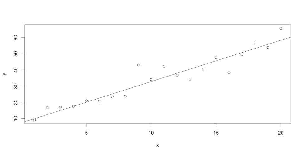
Pretty good fit! Let’s see how that compares to ordinary least squares regression, as computed by R.
>lm (y~x)Call:lm(formula = y ~ x)Coefficients:(Intercept) x8.402 2.491
The least squares result is in red. Pretty close too! Finally, let me add the true line in blue with the slope and intercept values I used to generate the test dataset, 2.38 and 8.29.

Note that in my example there’s only one place where Nelder-Mead is mentioned. That’s because the optimize package is abstracted enough that I can easily swap out the actual algorithm. Overall, I think the optimize package is very well organized and easy to work with, and I look forward to trying out more of the gonum collection!


