If you’re a programmer or computer scientist, you’re probably familiar with Big-O notation. It’s part of your foundational understanding of how complex a problem and/or algorithm is. But most explanations of Big-O notation [overcomplicate][1] what’s actually a very simple subject, and make it inaccessible to a larger audience who needs a common vocabulary and understanding of this important concept.

Breaking Down Big-O Notation
The first thing to remember is that Big-O notation is just a fancy way of stating what’s intuitive common sense for pretty much everyone already. The O stands for “order”, and you can think of it in English as a way of saying “this algorithm costs on the order of X to run.” You usually write this as O(X) and say it out loud as “order X”. Here I’m using X as a placeholder, and now I’ll explain what can go into that placeholder.
The Size Of The Problem
Big-O notation needs to be understood in relationship to the size of the problem you’re trying to solve. The classic example is sorting a list of numbers. The size of the problem is the length of the list, in this case. Big-O notation expresses how complex a sorting algorithm is relative to the length of the list to sort.
However, the length of the list is not used explicitly in the notation, but rather is replaced by a variable, usually N. We usually place an equation involving N inside the parentheses, for example,
O( log N )
Algorithmic Cost
Now if we’re looking at a particular method (algorithm) of sorting a list of numbers, we can talk quickly about how efficient (costly) it is to execute for a given list size.
The stereotypical bad algorithm for sorting is bubble-sort. The number of operations required to sort the list with bubble-sort grows much faster than the size of the list. In fact, if you double the list size, you might multiply the number of operations by up to four, and if you triple the list size, it might cost as much as nine times as many operations to sort the list.
We express this complexity by saying the cost grows in relationship to N squared, or:
Bubble-sort is O(N*N)
In English, we’d say that out loud as “bubble-sort is order N squared.”
Asymptotic Complexity and Upper Bounds
There are a few subtleties to keep in mind. All of these are really just generalizations that allow you to casually speak about algorithms without being very specific, with a wave of the hand, and yet get to the essence of their performance.
- Big-O notation really means that the problem can be “as bad as” the equation inside the parentheses. It’s an upper bound — a worst-case scenario.
- Big-O notation is expressed as the limiting factor as the size of the problem grows “very large.” Thus, even if at a small size the algorithm’s cost is dominated by a huge initial cost, what we’re interested in is what happens as the size goes to infinity.
- If there are multiple types of algorithmic costs, we disregard all but the worst as size goes to infinity, because eventually it will dwarf all other factors.
To give some real examples of this, many algorithms have one or more portions that are more-or-less dominated by the following types of costs:
- Constant cost. No matter how big the problem is, the algorithm requires exactly the same number of operations to complete.
- Logarithmic cost. As the problem grows, the cost grows logarithmically.
- Linear cost. Cost grows as a constant multiple of the problem size.
- Quadratic cost, as illustrated by bubble-sort above.
- Exponential cost. The Tower of Hanoi problem is a good example: to solve a Tower of Hanoi with N disks, you have to move the disks 2-raised-to-the-N-power times.
- Factorial cost. This is really bad!
There are other types of cost, but that covers the usual suspects, in order of increasing badness.
The Order Of Cost
Now, here’s the key thing. All we care about is which of these cost factors is worst as the problem size grows to infinity. And we care about the
order of that cost, disregarding constant factors that multiply it or add to it. In Computer Science courses you spend a lot of time proving to the professor (who already knows, we presume) that as the problem grows to infinity, an O(N*N) algorithm is eventually worse than an O(log N) algorithm.
To state this concretely, suppose we have a sort algorithm (let’s call it Baron-Sort) that takes 10 operations of startup cost to prepare, and for every element in the list to be sorted, it takes an additional 5 operations per element. Plus, as the list size N grows, it costs an additional N(N-1) operations.
We also have a Kyle-Sort algorithm that requires 100000 operations of setup cost, 50 operations per element, and its complexity grows as N(log(N)) in the size of the problem.
Baron-Sort = 10 + 5N * (N-1) Kyle-Sort = 100000 + 50N * (log N)
Which is better? It sort of looks like Baron-Sort is better, doesn’t it? But that’s only because of the small constant factors. As the problem gets really big, the influence of those constant factors becomes asymptotically meaningless, and we can disregard them. So the real complexity of the algorithms is quite different. Simplifying and clarifying:
Baron-Sort = N * N Kyle-Sort = N * log N
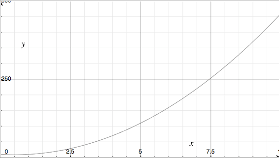
To illustrate this graphically, let’s plot the two equations, constants and all. Here’s Baron-sort and Kyle-sort. Whoa, look, Kyle-sort is literally off the chart! Looks like Baron-sort is much better, right?
But what happens when we start sorting really large lists? Let’s zoom out.
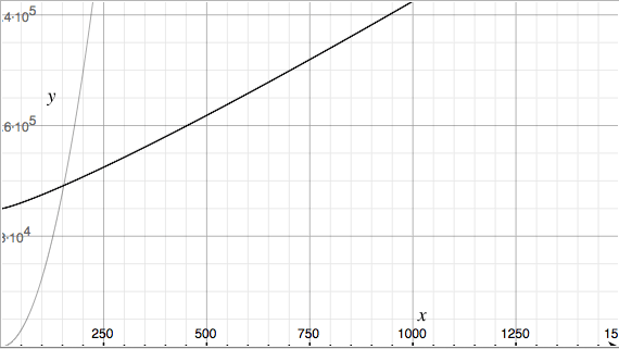
Now we can see that although Kyle-sort starts out with much worse initial cost, it grows much more slowly.
And that’s what Big-O notation is really about. Ignore the constant costs, and figure out what’ll grow fastest as the problem size grows. That cost eventually dominates in the long term,
no matter how big the constant factors are.
Here’s another example. If the equation for the cost of the algorithm is 100N^3 + 42N^2 + 2N, the fastest-growing component of that equation is all that matters. The algorithm is “order N cubed.” That’s all you need to know for Big-O notation.
Problem Complexity
Some problems have a built-in complexity, regardless of the algorithm used. For example, sorting again. We generally accept that the best any algorithm can ever do is O(N log N). Sorting itself is inherently that complex and can’t be made faster. So we can use Big-O notation to talk about the problem’s complexity as well as the complexity of solutions to the problem.
Big-O notation is really just a communication tool. It’s designed so that we can all shortcut the tedious and wordy explanations of how expensive an algorithm is and say, in the long run, it’s more or less about the same as some equation or other.
It’s a fairly blunt instrument in the real world, however. Many sort algorithms have best-case, ordinary-case, and worst-case behaviors. For example, a list that’s already sorted can be verified in a trivial O(N) operation. Constant factors and fixed setup costs matter, too. That’s because we’re usually not sorting infinitely large lists. Many systems use one algorithm or another because of specific costs that tend to be more or less for the problem domain most commonly seen, or other behaviors of the algorithms that may be desirable or undesirable.
But for dispensing with wordy discussions like the above, nothing beats “order N log N” as a way to quickly communicate a lot of the essence of a problem or algorithm. Hopefully this article helps you understand Big-O notation and/or explain it to someone else!